Starting from version 0.9.1 of the pvlib-python library, the development of the energy yield forecasting module for photovoltaic installations based on weather data from a wide range of weather models has been discontinued. Unfortunately, the API interface to access the models has changed, and no one volunteered to adapt the pvlib.Forecast module. However, this does not mean that we cannot benefit from the existing achievements in this area and continue to enjoy the ability to use the forecasts available in Unidata based on the NOAA/NCEP/NWS (National Centers for Environmental Prediction) models, including the GFS (Global Forecast System). And that’s what this blog post is about – how to obtain information about the potential energy yield from our photovoltaic installation based on the NCEP weather forecast.
The GFS Model
The GFS (Global Forecast System) model was not chosen randomly because, as the name suggests, it has global coverage, including a forecast for Poland. Generally, GFS provides global atmospheric and wave forecasts with a resolution of 13 km. It is run four times a day and allows for generating forecasts in three-hour intervals up to 10 days and with a 12-hour interval for 10-16 day forecasts. More information about the GFS model can be found on the webpage.
The GFS model data (but not only that) is collected in the Unidata THREDDS catalog. In the Forecast Model Data catalog, you can find a range of forecasts developed using different models and with varying spatial resolution. Currently, we are interested in obtaining the weather forecast for the next 7 days using the half-degree GFS model.
The model stores a vast amount of information, including 170 different variables. For the purpose of forecasting energy yield from photovoltaic installations, we do not need all variables. We will focus only on the following ones:
- Temperature_surface
- u-component_of_wind_isobaric
- v-component_of_wind_isobaric
- Total_cloud_cover_entire_atmosphere_Mixed_intervals_Average
- Low_cloud_cover_low_cloud_Mixed_intervals_Average
- Medium_cloud_cover_middle_cloud_Mixed_intervals_Average
- High_cloud_cover_high_cloud_Mixed_intervals_Average
- Total_cloud_cover_boundary_layer_cloud_Mixed_intervals_Average
- Total_cloud_cover_convective_cloud
These variables represent ambient temperature, wind components for determining wind speed, and information about cloud cover.
To facilitate access to this data, Unidata has developed a library called siphon, which allows for programmatic access to THREDDS data. So, let’s get to work!
Weather Forecast from THREDDS
First, we read the appropriate catalog using the TDSCatalog() method. Then, we select the dataset, in this case, “Best GFS Half Degree Forecast Time Series,” and open remote access to the data using the subset() method.
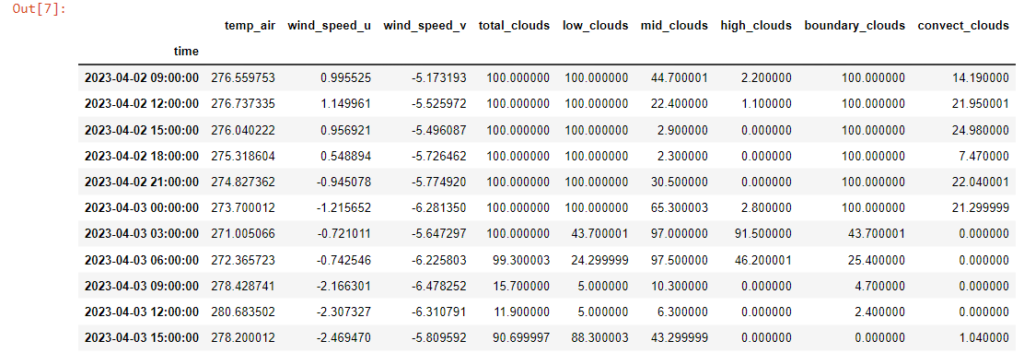
n the next steps, we prepare a request to the NCSS service to retrieve the data for the aforementioned variables. We also specify the geographical location, elevation, and the forecast period. This way, we create a data frame, df
Currently, I will convert the forecasted cloud cover into radiation components because, as it seems, such information is not directly available in the structure of the weather forecast data. For this purpose, I will use the code developed within the existing pvlib.forecast module, which I have slightly modified. The complete code can be found on the Github server.
The pvlib-python library provides two basic methods for converting cloud cover forecasts into irradiance forecasts. One method assumes a linear relationship between cloud cover and GHI (Global Horizontal Irradiance), meaning it applies scaling to the clear-sky climatology and then uses the DISC model to calculate DNI (Diffuse Horizontal Irradiance). The second method assumes a linear relationship between cloud cover and atmospheric transmittance, and then uses the Campbell-Normana model to calculate the components of GHI, DNI, and DHI [1]. Campbell-Normana is an approximation of the Liu-Jordan model [2].
Returning to our dataset for a moment, please note that the model generates data with a 3-hour time resolution. Therefore, if we want to obtain a bit more detail, we need to interpolate the forecasted data and accept certain errors associated with this process. However, using the interpolate() function from the pandas library makes it easy to interpolate the cloud cover forecast onto a time domain with higher resolution.
As a result of interpolation with an hourly resolution, we obtain data based on which we analyze the energy yield from a photovoltaic installation.
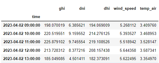
And finally, a graphical representation of the forecasted components of solar irradiance.

Links:
- Campbell, G. S., J. M. Norman (1998) An Introduction to Environmental Biophysics. 2nd Ed. New York: Springer
- B. Y. Liu and R. C. Jordan, The interrelationship and characteristic distribution of direct, diffuse, and total solar radiation, Solar Energy 4, 1 (1960)
- Downloading model fields with NCSS